Figure 1: Artwork by @allison_horst.
TL; DR
This post was updated on 2022-07-05 as updates in from
gtsummary 1.5.1 to 1.6.1 greatly streamlined exporting
summary tables to pdf.
Customizing tables in PDF output is possible with {knitr}
, {kableExtra} and a bit of LaTeX.
Updates available in {gtsummary} 1.5.1 also allow users to
more easily take advantage of these features in summary tables.

Figure 2: Scrolling PDF of penguins report with custom tables.
Check out the source file for the Penguins Report and rendered results:
Packages
This material was developed using:
| Software / package | Version |
|---|---|
| R | 4.2.0 |
| RStudio | 351 “Ghost Orchid” |
rmarkdown |
2.11 |
knitr |
1.37 |
kableExtra |
1.3.4 |
tinytex |
0.34 |
gtsummary |
1.6.1 |
pandoc |
2.14.0.3 |
palmerpenguins |
0.1.0 |
Background
Can anyone point me to a good R package that can create tables that are easily outputted in PDF. So far every package I have found seems to require numerous external packages and plug-ins in order to output the table as a PDF document. Any advice welcome.
— Charlie Harper (@charlieharperuk) January 20, 2022
You and me both, Charlie! This is tricky. I tried to avoid the LaTeX
route through {pagedown} , but ultimately because I
had many tables that varied in size and length, this was not a quick
approach.
Here is a solution I have landed upon; I hope it helps you and others as well. If anyone has additional tips or approaches, please share in the comments!
For a comprehensive overview of the many reporting options available via RMarkdown, and how to customize them, check out the excellent 2021 RStudio webinar Business Reports with R Markdown by Christophe Dervieux.
Document Set-up
Here is the initial set up of my .Rmd document,
including the YAML, some knitr options, and some LaTeX
options.
---
title: "Penguins Report"
author: "Shannon Pileggi"
date: "`r Sys.Date()`"
output:
  pdf_document:
    toc: true
    toc_depth: 2
    number_sections: true
    keep_tex: yes
latex_engine: pdflatex
classoption: landscape
header-includes:
  \usepackage{helvet}
  \renewcommand\familydefault{\sfdefault}
include-before:
- '`\newpage{}`{=latex}'
---

\let\oldsection\section
\renewcommand\section{\clearpage\oldsection}

options(knitr.kable.NA = '')
YAML
keep_tex: yesThis can be useful for reviewing the tex output to troubleshoot errors. For more ideas on how to leverage this, check out the blog post Modifying R Markdown’s LaTeX styles by Travis Gerke.latex_engine: pdflatexThe LaTeX engine can be changed to take advantage of other LaTeX features; see R Markdown: The Definitive Guide Ch 3.3.7 Advanced Customization for details.classoption: landscapeChanges orientation from portrait to landscape for wide tables.header-includes: \usepackage{helvet} \renewcommand\familydefault{\sfdefault}Changes the default font from serif to sans serif.include-before: - '{=latex}'Creates a page break in between title page and table of contents.
LaTeX
\let\oldsection\section \renewcommand\section{\clearpage\oldsection}creates a page break for each new numbered top level section.
knitr options
options(knitr.kable.NA = '') displays blank instead of
NA for missing values.
Raw Data Tables
Default Column Names
Here are options I used to create a basic table with default column names.
penguins %>%
  knitr::kable(
    format = "latex",
    align = "l",
    booktabs = TRUE,
    longtable = TRUE,
    linesep = "",
    ) %>%
  kableExtra::kable_styling(
      position = "left",
      latex_options = c("striped", "repeat_header"),
      stripe_color = "gray!15"
    )
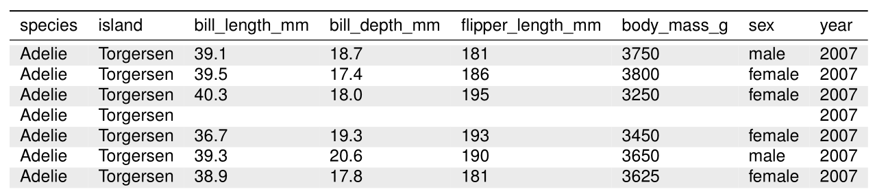
Figure 3: Raw data table PDF output with default column names.
Many of knitr::kable() arugments are passed as
... Other arguments, and are described in more
detail in the help file of kableExtra::kbl().
format = "latex"specifies the output format.align = "l"specifies column alignment.booktabs = TRUEis generally recommended for formatting LaTeX tables.longtable = TRUEhandles tables that span multiple pages.linesep = ""prevents default behavior of extra space every five rows.
Additional styling options are specified with
kableExtra::kable_styling().
position = "left"places table on left hand side of page.latex_options = c("striped", "repeat_header")implements table striping with repeated headers for tables that span multiple pages.stripe_color = "gray!15"species the stripe color using LaTeX color specification from the xcolor package - this specifies a mix of 15% gray and 85% white.
Custom Column Names
I was also interested in implementing column names with specific line
breaks, which is a bit more complicated. To achieve this, use both
col.names and escape = FALSE. Be cautious with
escape = FALSE as this may cause rendering errors if your
table contains special LaTeX characters like \ or
%.
# original column names
names(penguins)
[1] "species"           "island"            "bill_length_mm"
[4] "bill_depth_mm"     "flipper_length_mm" "body_mass_g"
[7] "sex"               "year"
#Create column names with line breaks for demonstration.
column_names <- penguins %>%
names() %>%
str_replace_all( "_", "\n")
column_names
[1] "species"             "island"              "bill\nlength\nmm"
[4] "bill\ndepth\nmm"     "flipper\nlength\nmm" "body\nmass\ng"
[7] "sex" "year" 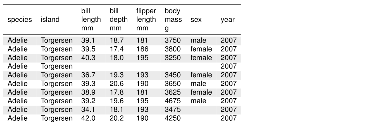
Figure 4: Raw data table PDF output with custom column names with line breaks.
Summary Data Tables
With the release of gtsummary 1.5.1, these print to pdf
features are now also available for summary tables through updates to gtsummary::as_kable_extra().
Default column names
Apply styling as desired with
gtsummary; for example, bold labels.Pass the same options to
gtsummary::as_kable_extra()that can be passed toknitr::kable()/kableExtra::kbl().Finish with additional
kableExtra::kable_styling()specifications.
penguins %>%
  gtsummary::tbl_summary(
    by = species
  ) %>%
  gtsummary::bold_labels() %>%
  gtsummary::as_kable_extra(
    format = "latex",
    booktabs = TRUE,
    longtable = TRUE,
    linesep = ""
    ) %>%
  kableExtra::kable_styling(
      position = "left",
      latex_options = c("striped", "repeat_header"),
      stripe_color = "gray!15"
    )
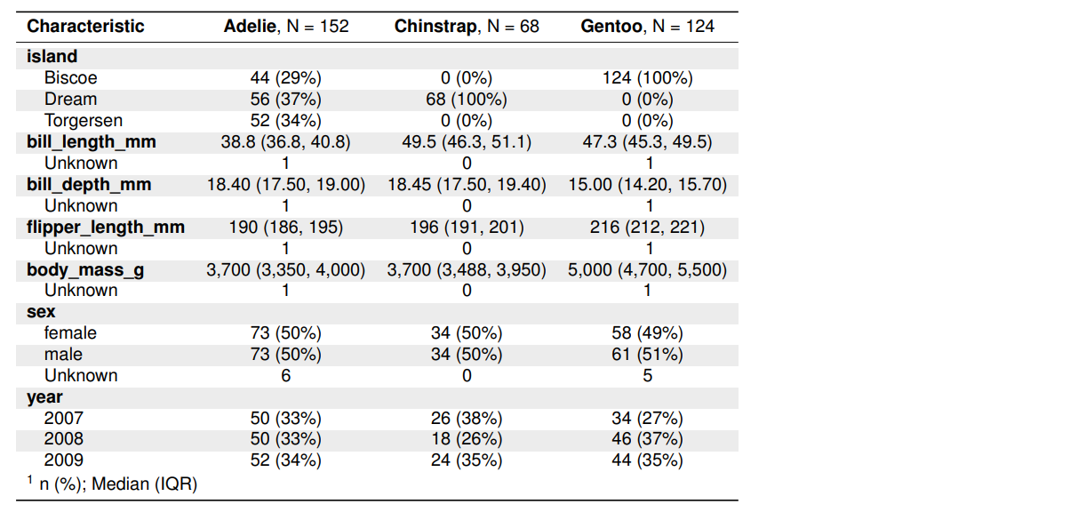
Figure 5: Summary tables PDF output with default column names.
Custom column names
When this post was originally published on 2022-01-24, this was
harder. Thanks to updates in gtsummary 1.6.1, custom column
names can now be implemented directly in modify_header()
and seamlessly rendered to pdf via kableExtra.
penguins %>%
  gtsummary::tbl_summary(
    by = species,
    statistic = list(all_categorical() ~ "{n} ({p}%)")
  ) %>%
  gtsummary::bold_labels() %>%
  gtsummary::modify_header(
    label = "**Characteristic**",
    all_stat_cols() ~ "**{level}**\nN = {n}"
  ) %>%
  gtsummary::as_kable_extra(
    format = "latex",
    booktabs = TRUE,
    longtable = TRUE,
    linesep = ""
    ) %>%
  kableExtra::kable_styling(
      position = "left",
      latex_options = c("striped", "repeat_header"),
      stripe_color = "gray!15"
    )
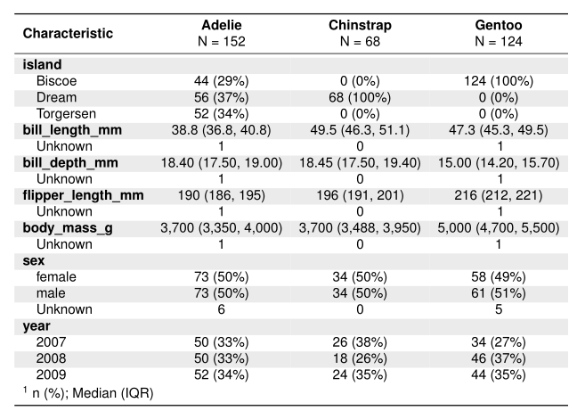
Figure 6: Summary tables PDF output with custom column names, including line breaks and bolding.
Summary
With a little bit of LaTeX and fairy dust 🧙, report ready PDF tables are possible. 🥂
Acknowledgements
Thank you Daniel Sjoberg for updating {gtsummary} to make printing to pdf more streamlined for summary tables! 🎉 And for kindly providing feedback on this post. Also, thanks to Travis Gerke for tips on leveraging LaTeX via rmarkdown.