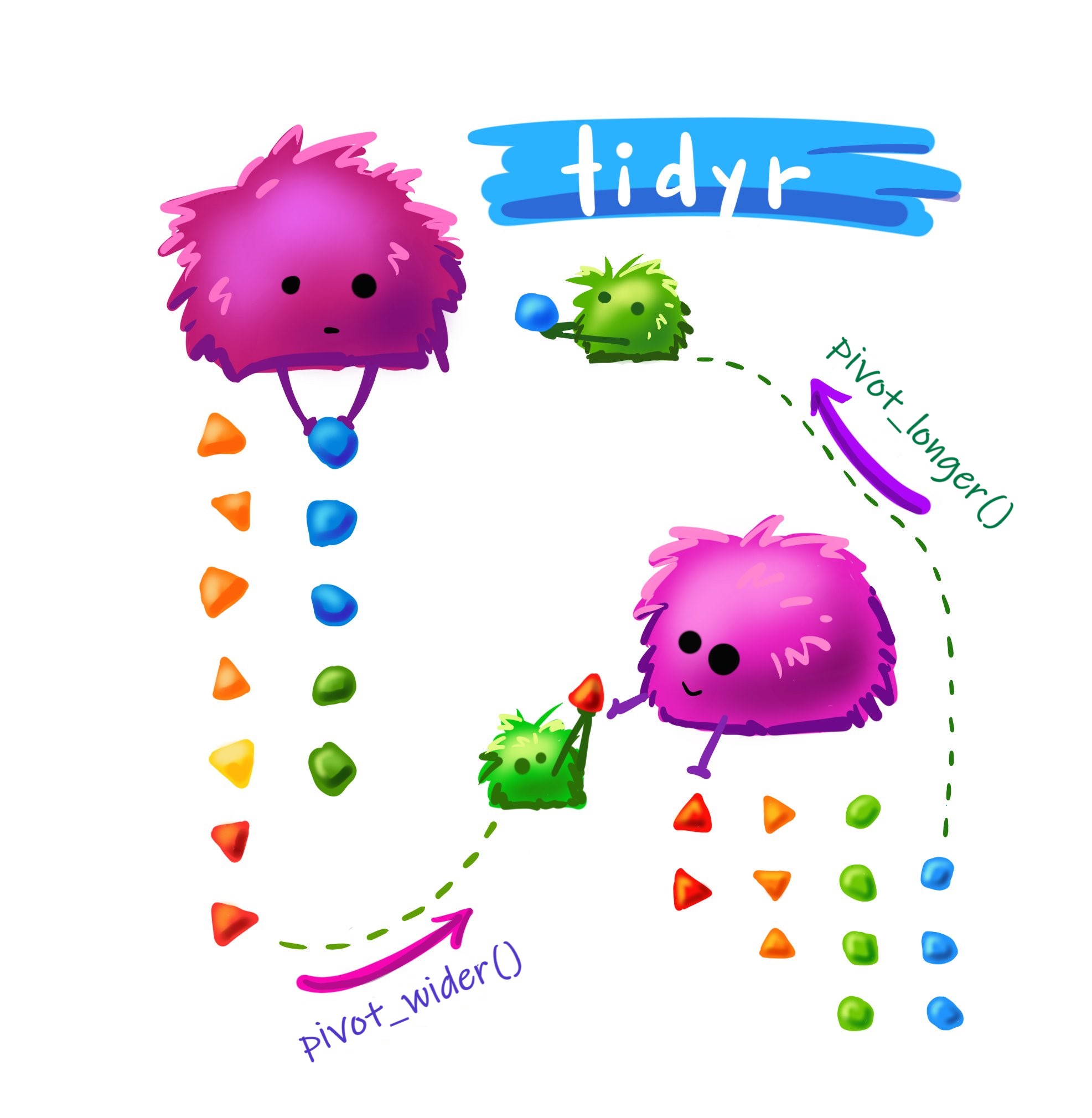
Figure 1: Artwork by @allison_horst, modified to substitute pivot_wider() and pivot_longer() for spread and gather.
TL; DR
I demonstrate a pivot_longer() plus pivot_wider() approach to data preparation as an alternative to explicitly coding computations. This approach might be beneficial for you if you have:
✅ wide data,
✅ with a consistent naming structure,
✅ and many variables to aggregate.
Background
I love reading and watching Julia Silge’s #TidyTuesday tidymodels tutorials! Recently I was following her post about xgboost classification models with the beach volleyball data. The first 15 minutes of the 50 minute video are about getting familiar with the data and preparing it for modeling, and I realized I would have taken a different approach to the data preparation involving pivot_longer() and pivot_wider(). Also, Spencer Zeigler recently tweeted asking about this approach.
do you ever have to pivot_longer() first to get pivot_wider() to do what you want? or is my data just formatted badly? or am I bad at pivoting data? or both? #rstats #tidyr
— Spencer Zeigler (@spenceometry) August 24, 2021
Yes Spencer, I do this all the time!
Getting started
This material was developed using:
| Software / package | Version |
|---|---|
| R | 4.0.5 |
| RStudio | 1.4.1103 |
tidyverse |
1.3.1 |
Import the data
#TidyTuesday provides more information about the beach volleyball data.
vb_matches <- readr::read_csv('https://raw.githubusercontent.com/rfordatascience/tidytuesday/master/data/2020/2020-05-19/vb_matches.csv', guess_max = 76000)
vb_matches
# A tibble: 76,756 x 65
   circuit tournament     country     year date       gender match_num
   <chr>   <chr>          <chr>      <dbl> <date>     <chr>      <dbl>
 1 AVP     Huntington Be~ United St~  2002 2002-05-24 M              1
 2 AVP     Huntington Be~ United St~  2002 2002-05-24 M              2
 3 AVP     Huntington Be~ United St~  2002 2002-05-24 M              3
 4 AVP     Huntington Be~ United St~  2002 2002-05-24 M              4
 5 AVP     Huntington Be~ United St~  2002 2002-05-24 M              5
 6 AVP     Huntington Be~ United St~  2002 2002-05-24 M              6
 7 AVP     Huntington Be~ United St~  2002 2002-05-24 M              7
 8 AVP     Huntington Be~ United St~  2002 2002-05-24 M              8
 9 AVP     Huntington Be~ United St~  2002 2002-05-24 M              9
10 AVP     Huntington Be~ United St~  2002 2002-05-24 M             10
# ... with 76,746 more rows, and 58 more variables: w_player1 <chr>,
#   w_p1_birthdate <date>, w_p1_age <dbl>, w_p1_hgt <dbl>,
#   w_p1_country <chr>, w_player2 <chr>, w_p2_birthdate <date>,
#   w_p2_age <dbl>, w_p2_hgt <dbl>, w_p2_country <chr>, w_rank <chr>,
#   l_player1 <chr>, l_p1_birthdate <date>, l_p1_age <dbl>,
#   l_p1_hgt <dbl>, l_p1_country <chr>, l_player2 <chr>,
#   l_p2_birthdate <date>, l_p2_age <dbl>, l_p2_hgt <dbl>,
#   l_p2_country <chr>, l_rank <chr>, score <chr>, duration <time>,
#   bracket <chr>, round <chr>, w_p1_tot_attacks <dbl>,
#   w_p1_tot_kills <dbl>, w_p1_tot_errors <dbl>,
#   w_p1_tot_hitpct <dbl>, w_p1_tot_aces <dbl>,
#   w_p1_tot_serve_errors <dbl>, w_p1_tot_blocks <dbl>,
#   w_p1_tot_digs <dbl>, w_p2_tot_attacks <dbl>,
#   w_p2_tot_kills <dbl>, w_p2_tot_errors <dbl>,
#   w_p2_tot_hitpct <dbl>, w_p2_tot_aces <dbl>,
#   w_p2_tot_serve_errors <dbl>, w_p2_tot_blocks <dbl>,
#   w_p2_tot_digs <dbl>, l_p1_tot_attacks <dbl>,
#   l_p1_tot_kills <dbl>, l_p1_tot_errors <dbl>,
#   l_p1_tot_hitpct <dbl>, l_p1_tot_aces <dbl>,
#   l_p1_tot_serve_errors <dbl>, l_p1_tot_blocks <dbl>,
#   l_p1_tot_digs <dbl>, l_p2_tot_attacks <dbl>,
#   l_p2_tot_kills <dbl>, l_p2_tot_errors <dbl>,
#   l_p2_tot_hitpct <dbl>, l_p2_tot_aces <dbl>,
#   l_p2_tot_serve_errors <dbl>, l_p2_tot_blocks <dbl>,
#   l_p2_tot_digs <dbl>
Original data preparation
This is copied straight from Julia’s blog post. The original data preparation involves writing formulas with transmute() followed by stacking data for winners and losers with bind_rows().
vb_parsed <- vb_matches %>%
  transmute(
    circuit,
    gender,
    year,
    w_attacks = w_p1_tot_attacks + w_p2_tot_attacks,
    w_kills = w_p1_tot_kills + w_p2_tot_kills,
    w_errors = w_p1_tot_errors + w_p2_tot_errors,
    w_aces = w_p1_tot_aces + w_p2_tot_aces,
    w_serve_errors = w_p1_tot_serve_errors + w_p2_tot_serve_errors,
    w_blocks = w_p1_tot_blocks + w_p2_tot_blocks,
    w_digs = w_p1_tot_digs + w_p2_tot_digs,
    l_attacks = l_p1_tot_attacks + l_p2_tot_attacks,
    l_kills = l_p1_tot_kills + l_p2_tot_kills,
    l_errors = l_p1_tot_errors + l_p2_tot_errors,
    l_aces = l_p1_tot_aces + l_p2_tot_aces,
    l_serve_errors = l_p1_tot_serve_errors + l_p2_tot_serve_errors,
    l_blocks = l_p1_tot_blocks + l_p2_tot_blocks,
    l_digs = l_p1_tot_digs + l_p2_tot_digs
  ) %>%
  na.omit()

winners <- vb_parsed %>%
  select(circuit, gender, year,
         w_attacks:w_digs) %>%
  rename_with(~ str_remove_all(., "w_"), w_attacks:w_digs) %>%
  mutate(win = "win")

losers <- vb_parsed %>%
  select(circuit, gender, year,
         l_attacks:l_digs) %>%
  rename_with(~ str_remove_all(., "l_"), l_attacks:l_digs) %>%
  mutate(win = "lose")

vb_df <- bind_rows(winners, losers) %>%
  mutate_if(is.character, factor)
vb_df
# A tibble: 28,664 x 11
   circuit gender  year attacks kills errors  aces serve_errors blocks
   <fct>   <fct>  <dbl>   <dbl> <dbl>  <dbl> <dbl>        <dbl>  <dbl>
 1 AVP     M       2004      45    24      7     0            2      5
 2 AVP     M       2004      71    31     16     3            8      7
 3 AVP     M       2004      43    26      5     2            4      7
 4 AVP     M       2004      42    32      5     2            3      7
 5 AVP     M       2004      44    31      1     0            5      6
 6 AVP     M       2004      55    31      6     0            4      8
 7 AVP     M       2004      39    26      8     5            3      4
 8 AVP     M       2004      41    21      8     1            1      6
 9 AVP     M       2004      60    33     12     0            1      9
10 AVP     M       2004      32    11      5     1            5      8
# ... with 28,654 more rows, and 2 more variables: digs <dbl>,
#   win <fct>
Alternative data preparation
This approach leverages pivot_wider() and pivot_longer() to avoid writing out explicit computations. This can work well if you need to aggregate many variables with a sum or a mean. This approach does require a unique identifier for each record.
vb_df <- vb_matches  %>%
  mutate(id = row_number()) %>%
  dplyr::select(
    id, circuit, gender, year,
    matches("attacks|kills|errors|aces|blocks|digs")
    ) %>%
  drop_na() %>%
  pivot_longer(
    cols = -c(id, circuit, gender, year),
    names_to = c("status", "player", "method", "metric"),
    names_pattern = "([wl])_(p[12])_(tot)_(.*)",
    values_to = "value"
  ) %>%
  group_by(id, circuit, gender, year, status, metric) %>%
  summarize(total = sum(value)) %>%
  ungroup() %>%
  pivot_wider(
    names_from = "metric",
    values_from = total
    )
And here is what the final data looks like!
vb_df
# A tibble: 28,664 x 12
      id circuit gender  year status  aces attacks blocks  digs errors
   <int> <chr>   <chr>  <dbl> <chr>  <dbl>   <dbl>  <dbl> <dbl>  <dbl>
 1  1846 AVP     M       2004 l          1      57      2    17     17
 2  1846 AVP     M       2004 w          0      45      5    11      7
 3  1847 AVP     M       2004 l          0      61      5    23     13
 4  1847 AVP     M       2004 w          3      71      7    21     16
 5  1848 AVP     M       2004 l          1      36      2    11      7
 6  1848 AVP     M       2004 w          2      43      7    10      5
 7  1849 AVP     M       2004 l          0      41      4    12      8
 8  1849 AVP     M       2004 w          2      42      7     7      5
 9  1850 AVP     M       2004 l          1      45      1     7      6
10  1850 AVP     M       2004 w          0      44      6    15      1
# ... with 28,654 more rows, and 2 more variables: kills <dbl>,
#   serve_errors <dbl>
In case that was hard to follow in one long code chunk, below I show what the data looks like at each of four steps annotated with comments.
Step 1: initial manipulation of wide data
# step 1: initial manipulation of wide data ----
step1 <- vb_matches  %>%
  # create unique identifier ----
  mutate(id = row_number()) %>%
  # retain relevant variables ----
  dplyr::select(
    id, circuit, gender, year,
    matches("attacks|kills|errors|aces|blocks|digs")
    ) %>%
  # remove records where any observations are missing ----
  drop_na()
step1
# A tibble: 14,332 x 32
      id circuit gender  year w_p1_tot_attacks w_p1_tot_kills
   <int> <chr>   <chr>  <dbl>            <dbl>          <dbl>
 1  1846 AVP     M       2004               11              6
 2  1847 AVP     M       2004               32             13
 3  1848 AVP     M       2004               19             11
 4  1849 AVP     M       2004               19             13
 5  1850 AVP     M       2004               24             21
 6  1851 AVP     M       2004               20              7
 7  1852 AVP     M       2004               17             11
 8  1853 AVP     M       2004                7              2
 9  1854 AVP     M       2004               16             10
10  1855 AVP     M       2004               13              5
# ... with 14,322 more rows, and 26 more variables:
#   w_p1_tot_errors <dbl>, w_p1_tot_aces <dbl>,
#   w_p1_tot_serve_errors <dbl>, w_p1_tot_blocks <dbl>,
#   w_p1_tot_digs <dbl>, w_p2_tot_attacks <dbl>,
#   w_p2_tot_kills <dbl>, w_p2_tot_errors <dbl>, w_p2_tot_aces <dbl>,
#   w_p2_tot_serve_errors <dbl>, w_p2_tot_blocks <dbl>,
#   w_p2_tot_digs <dbl>, l_p1_tot_attacks <dbl>,
#   l_p1_tot_kills <dbl>, l_p1_tot_errors <dbl>, l_p1_tot_aces <dbl>,
#   l_p1_tot_serve_errors <dbl>, l_p1_tot_blocks <dbl>,
#   l_p1_tot_digs <dbl>, l_p2_tot_attacks <dbl>,
#   l_p2_tot_kills <dbl>, l_p2_tot_errors <dbl>, l_p2_tot_aces <dbl>,
#   l_p2_tot_serve_errors <dbl>, l_p2_tot_blocks <dbl>,
#   l_p2_tot_digs <dbl>
Step 2: reshape data to long
# step 2: reshape data to long ----
step2 <- step1 %>%
  pivot_longer(
    # specify variables to hold fixed and not pivot ----
    cols = -c(id, circuit, gender, year),
    # create four new variables extracted from the variable name ----
    names_to = c("status", "player", "method", "metric"),
    # regex pattern to extract values from variable name ---
    names_pattern = "([wl])_(p[12])_(tot)_(.*)",
    # the value of the metric ---
    values_to = "value"
  )
step2
# A tibble: 401,296 x 9
      id circuit gender  year status player method metric       value
   <int> <chr>   <chr>  <dbl> <chr>  <chr>  <chr>  <chr>        <dbl>
 1  1846 AVP     M       2004 w      p1     tot    attacks         11
 2  1846 AVP     M       2004 w      p1     tot    kills            6
 3  1846 AVP     M       2004 w      p1     tot    errors           1
 4  1846 AVP     M       2004 w      p1     tot    aces             0
 5  1846 AVP     M       2004 w      p1     tot    serve_errors     1
 6  1846 AVP     M       2004 w      p1     tot    blocks           0
 7  1846 AVP     M       2004 w      p1     tot    digs             7
 8  1846 AVP     M       2004 w      p2     tot    attacks         34
 9  1846 AVP     M       2004 w      p2     tot    kills           18
10  1846 AVP     M       2004 w      p2     tot    errors           6
# ... with 401,286 more rows
Step 3: sum values of player 1 and player 2 for all metrics
# step 3: sum values of player 1 and player 2 for all metrics ----
step3 <- step2 %>%
  group_by(id, circuit, gender, year, status, metric) %>%
  summarize(total = sum(value)) %>%
  ungroup()
step3
# A tibble: 200,648 x 7
      id circuit gender  year status metric       total
   <int> <chr>   <chr>  <dbl> <chr>  <chr>        <dbl>
 1  1846 AVP     M       2004 l      aces             1
 2  1846 AVP     M       2004 l      attacks         57
 3  1846 AVP     M       2004 l      blocks           2
 4  1846 AVP     M       2004 l      digs            17
 5  1846 AVP     M       2004 l      errors          17
 6  1846 AVP     M       2004 l      kills           31
 7  1846 AVP     M       2004 l      serve_errors     5
 8  1846 AVP     M       2004 w      aces             0
 9  1846 AVP     M       2004 w      attacks         45
10  1846 AVP     M       2004 w      blocks           5
# ... with 200,638 more rows
Step 4: reshape data to wide for modeling
# step 4: reshape data to wide for modeling ----
step4 <- step3 %>%
  pivot_wider(
    names_from = "metric",
    values_from = total
    )
# A tibble: 28,664 x 12
      id circuit gender  year status  aces attacks blocks  digs errors
   <int> <chr>   <chr>  <dbl> <chr>  <dbl>   <dbl>  <dbl> <dbl>  <dbl>
 1  1846 AVP     M       2004 l          1      57      2    17     17
 2  1846 AVP     M       2004 w          0      45      5    11      7
 3  1847 AVP     M       2004 l          0      61      5    23     13
 4  1847 AVP     M       2004 w          3      71      7    21     16
 5  1848 AVP     M       2004 l          1      36      2    11      7
 6  1848 AVP     M       2004 w          2      43      7    10      5
 7  1849 AVP     M       2004 l          0      41      4    12      8
 8  1849 AVP     M       2004 w          2      42      7     7      5
 9  1850 AVP     M       2004 l          1      45      1     7      6
10  1850 AVP     M       2004 w          0      44      6    15      1
# ... with 28,654 more rows, and 2 more variables: kills <dbl>,
#   serve_errors <dbl>
Summary
If you are fortunate enough to have wide data with a consistent naming structure, using a pivot_longer() / pivot_wider() data preparation approach can save you from writing out tedious formulas. Let me know what you think!