TL;DR
To kick off my week curating the @WeAreRLadies twitter account I created a gif to introduce myself using gganimate and ggtext.
Getting started
This material was developed using:
| Software / package | Version |
|---|---|
| R | 4.0.3 |
| RStudio | 1.4.1103 |
tidyverse |
1.3.0 |
gganimate |
1.0.7 |
extrafont |
0.17 |
ggtext |
0.1.1 |
glue |
1.4.1 |
Fonts
Fonts were challenging for me to get started with in R, and I got some great tips on twitter. I ended up manually installing new fonts on my Windows 10 OS and then using the extrafont package to access the fonts in R.
# import fonts; only needed one time or after new font installation ----
# fonts may install to multiple directories; figure out where yours are installed ----
# and adjust path accordingly if needed ----
# this can take a while ----
extrafont::font_import()

# do this each R session in which you want to use fonts ----
extrafont::loadfonts(device = "win")

# examine font family names available for use (output not shown) ----
extrafont::fonts()
The data
The data needed to create a map of the US is already contained within ggplot2.
us_states <- ggplot2::map_data("state")
To show locations where I have lived, I manually compiled a data frame with city, state, latitude, longitude, and a description.
# use <br> to render line breaks with ggtext ----
residence <- tribble(
  ~city,           ~state,  ~lat,   ~long, ~years, ~description,
  "Raleigh",         "NC", 35.82,  -78.66,  17,    "Childhood",
  "Greenville",      "NC", 35.60,  -77.37,   4,    "Undergrad at ECU",
  "Atlanta",         "GA", 33.76,  -84.42,  10,    "Grad school at Emory<br>Statistician at CDC<br>Lecturer at Emory",
  "San Luis Obispo", "CA", 35.28, -120.66,   3,    "Asst. Professor at Cal Poly SLO",
  "Williamsburg",    "VA", 37.27,  -76.71, 0.5,    "Time with family",
  "Doylestown",      "PA", 40.31,  -75.13,   2,    "Statistician at Adelphi Research"
)
Then I needed to create a transition state for gganimate (city_order) as well as indicate connections between residences for the arrows.
residence_connections_prelim <- residence %>%
  mutate(
    # need this to create transition state ----
    city_order = row_number() + 1,
    # where I moved to next, for curved arrows ----
    lat_next = lead(lat),
    long_next = lead(long),
    # label to show in plot, styled using ggtext ---
    label = glue::glue("**{city}, {state}** ({years} yrs)<br>*{description}*"),
    # label of next location ----
    label_next = lead(label)
  )
Lastly, I modified this data a bit so that the first residence shows the label at the residence with no arrow and all remaining residences show an arrow with the label positioned at the next residence.
residence_connections <- residence_connections_prelim %>%
  # get first row of residence ----
  slice(1) %>%
  # manually modify for plotting ----
  mutate(
    city_order = 1,
    label_next = label,
    lat_next = lat,
    long_next = long,
    ) %>%
  # combine with all other residences ----
  bind_rows(residence_connections_prelim) %>%
  # last (7th) row irrelevant ----
  slice(1:6) %>%
  # keep what we neeed ----
  dplyr::select(city_order, lat, long, lat_next, long_next, label_next)
residence_connections
# A tibble: 6 x 6
  city_order   lat   long lat_next long_next label_next
       <dbl> <dbl>  <dbl>    <dbl>     <dbl> <glue>
1          1  35.8  -78.7     35.8     -78.7 **Raleigh, NC** (17 yrs)~
2          2  35.8  -78.7     35.6     -77.4 **Greenville, NC** (4 yr~
3          3  35.6  -77.4     33.8     -84.4 **Atlanta, GA** (10 yrs)~
4          4  33.8  -84.4     35.3    -121.  **San Luis Obispo, CA** ~
5          5  35.3 -121.      37.3     -76.7 **Williamsburg, VA** (0.~
6          6  37.3  -76.7     40.3     -75.1 **Doylestown, PA** (2 yr~
Base map
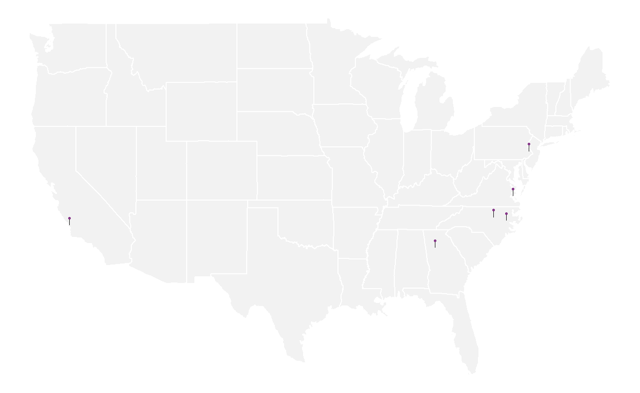
For the map itself, I created a base map showing pins of the locations I have lived. Hex codes for R-Ladies colors were obtained from this blog post by Alison Hill. I briefly experimented with coord_map for projection, but then the subsequent curved arrows presented incorrectly.
base_map <- ggplot() +
  # plot states ----
  geom_polygon(
    data = us_states,
    aes(
      x     = long,
      y     = lat,
      group = group
      ),
    fill  = "#F2F2F2",
    color = "white"
  ) +
  # lines for pins ----
  geom_segment(
    data = residence,
    aes(
      x    = long,
      xend = long,
      y    = lat,
      yend = lat + 0.5
      ),
    color = "#181818",
    size = 0.3
    ) +
    # pin heads, a bit above actual location, color with R ladies lighter purple ----
  geom_point(
    data = residence,
    aes(
      x = long,
      y = lat + 0.5
      ),
    size = 0.5,
    color = "#88398A"
  ) +
  theme_void()
The sizing of the pins in the base_map appears different than in the gif below as increasing the resolution of the output gif alters plotting ratios.
base_map
Animated map
anim <- base_map +
  # show arrows connecting residences ----
  geom_curve(
    # do not include 1st residence in arrows as no arrow is intended ----
    # and inclusion messes up transition ---
    data = residence_connections %>% slice(-1),
    # add slight adjustment to arrow positioning ----
    aes(
      y     = lat - 0.1,
      x     = long,
      yend  = lat_next - 0.2,
      xend  = long_next,
      # group is used to create the transition ----
      group = seq_along(city_order)
    ),
    color = "#181818",
    curvature = -0.5,
    arrow = arrow(length = unit(0.02, "npc")),
    size  = 0.2
  ) +
  # add in labels for pins, with inward positioning ----
  # show labels either top left or top right of pin ----
  geom_richtext(
    data = residence_connections,
    aes(
      x     = ifelse(long_next < -100, long_next + 1, long_next - 1),
      y     = lat_next + 5,
      label = label_next,
      vjust = "top",
      hjust = ifelse(long_next < -100, 0, 1),
      # group is used to create the transition ----
      group = seq_along(city_order)
    ),
    size = 2,
    label.colour = "white",
    # R ladies purple ----
    color = "#562457",
    # R ladies font used in xaringan theme ----
    family = "Lato"
  ) +
  # title determined by group value in transition ----
  ggtitle("Home {closest_state} of 6") +
  # create animation ----
  transition_states(
    city_order,
    transition_length = 2,
    state_length = 5
    ) +
  # style title ----
  theme(
    plot.title = element_text(
      color = "#562457",
      family = "Permanent Marker",
      size = 12
      )
    )
# render and save transition ----
# the default nframes 100 frames, 150 makes the gif a bit longer for readability ----
# changing dimensions for output w/ height & width ----
# increasing resolution with res ----
animate(anim, nframes = 150, height = 2, width = 3, units = "in", res = 150)
anim_save("homes_animation.gif")
Discussion
I hope this gif helped you learn a little bit about me! I’m a southern girl who was never quite cool enough for California still learning how to navigate personalities in the northeast. 😂
I do have two additional short-term residences not shown here. Although I was born in Raleigh, NC, I lived in Accra, Ghana until I was 1 year old (my father served in the US military and worked at the American Embassy in Accra). I also lived in Seville, Spain for a semester abroad during college.
In this gif I did not include transitions between countries (because, you know, I’m a parent working in a pandemic and I have to draw the line on my free time somewhere). In addition, aligning sizing with resolution of the output device took some experimentation.
I would love to get to know you through your gif - if you happen to replicate this for yourself please share with me on Twitter, LinkedIn, or email! I also invite you to improve this gif with cooler transitions, international locations, awesome styles, or anything else. 😀 💜